Example of 2D Convolution

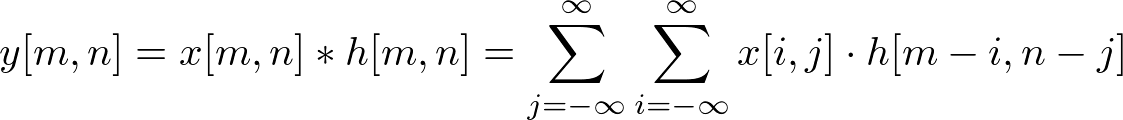
Here is a simple example of convolution of 3x3 input signal and impulse response (kernel) in 2D spatial. The definition of 2D convolution and the method how to convolve in 2D are explained in the main page, and it also explaines why the kernel is flipped.

In general, the size of output signal is getting bigger than input signal (Output Length = Input Length + Kernel Length - 1), but we compute only same area as input has been defined. Because we forced to pad zeros where inputs are not defined, such as x[-1,-1], the results around the edge cannot be accurate. Plus, the size of output is fixed as same as input size in most image processing.

Notice that the origin of impulse response is always centered. (h[0,0] is located at the center sample of kernel, not the first element.)

Let's start calculate each sample of the output one by one.
First, flip the kernel, which is the shaded box, in both horizontal and vertical direction. Then, move it over the input array. If the kernel is centered (aligned) exactly at the sample that we are interested in, multiply the kernel data by the overlapped input data.
The accumulation (adding these 9 multiplications) is the last thing to do to find out the output value.

Note that the matrices are referenced here as [column, row], not [row, column]. M is horizontal (column) direction and N is vertical (row) direction.

---

---

---

---

---

---

---

---